Multi-Tumour Analysis and Sensitivity Analyses with seerSurv

Sameer Mansoori, Shubhram Pandey, Rashi Rani, Barinder Singh, Murat Kurt

2026-03-21

Overview

This vignette demonstrates the batch analysis workflow for all 11 cancer types in the bundled tumour_data_seer dataset across all supported time horizons ("lifetime", "20y", "5y") and both information criteria ("AIC", "BIC").

library(seerSurv)
library(dplyr)
library(tidyr)
library(ggplot2)

---

Load bundled datasets

data(lifetable_seer)
data(tumour_data_seer)

dplyr::glimpse(tumour_data_seer)
#> Rows: 22
#> Columns: 12
#> $ Tumor      <chr> "Kidney", "Kidney", "Bladder", "Bladder", "Ovarian", "Ovari…
#> $ Recurrence <chr> "LR", "DR", "LR", "DR", "LR", "DR", "LR", "DR", "LR", "DR",…
#> $ S0         <dbl> 1, 1, 1, 1, 1, 1, 1, 1, 1, 1, 1, 1, 1, 1, 1, 1, 1, 1, 1, 1,…
#> $ S1         <dbl> 0.9750000, 0.4856000, 0.8898000, 0.3517000, 0.9523000, 0.77…
#> $ S2         <dbl> 0.9559000, 0.3427000, 0.8103000, 0.1943000, 0.9103000, 0.62…
#> $ S3         <dbl> 0.9376000, 0.2668000, 0.7660000, 0.1415000, 0.8798000, 0.50…
#> $ S4         <dbl> 0.9212000, 0.2245000, 0.7359000, 0.1189000, 0.8476000, 0.41…
#> $ S5         <dbl> 0.9049000, 0.1895000, 0.7123000, 0.1037000, 0.8186000, 0.34…
#> $ prop_male  <dbl> 0.649, 0.712, 0.790, 0.735, 0.000, 0.000, 0.000, 0.000, 0.4…
#> $ mean_age   <dbl> 61, 62, 65, 64, 59, 62, 61, 61, 65, 64, 63, 63, 63, 63, 61,…
#> $ N_LR       <int> 11495, 11495, 6840, 6840, 6460, 6460, 93100, 93100, 17575, …
#> $ N_DR       <int> 605, 605, 360, 360, 340, 340, 4900, 4900, 925, 925, 155, 15…

---

Run all scenarios

scenarios <- c("lifetime", "20y", "5y")
criteria  <- c("AIC", "BIC")

run_batch <- function(scen, crit) {
  tumour_data_seer |>
    group_by(Tumor) |>
    summarise(
      out = list(
        run_tumour_analysis(
          tumour       = first(Tumor),
          surv_vec_LR  = c(S0[Recurrence == "LR"], S1[Recurrence == "LR"],
                           S2[Recurrence == "LR"], S3[Recurrence == "LR"],
                           S4[Recurrence == "LR"], S5[Recurrence == "LR"]),
          surv_vec_DR  = c(S0[Recurrence == "DR"], S1[Recurrence == "DR"],
                           S2[Recurrence == "DR"], S3[Recurrence == "DR"],
                           S4[Recurrence == "DR"], S5[Recurrence == "DR"]),
          N_L          = first(N_LR),
          N_D          = first(N_DR),
          prop_male_LR = prop_male[Recurrence == "LR"],
          mean_age_LR  = mean_age[Recurrence == "LR"],
          prop_male_DR = prop_male[Recurrence == "DR"],
          mean_age_DR  = mean_age[Recurrence == "DR"],
          lifetable    = lifetable_seer,
          scenario     = scen,
          criterion    = crit
        )
      ),
      .groups = "drop"
    ) |>
    unnest(out) |>
    mutate(scenario = scen, criterion = crit)
}

all_results <- bind_rows(
  lapply(scenarios, function(s)
    lapply(criteria, function(c) run_batch(s, c)) |> bind_rows()
  )
)

dim(all_results)
#> [1] 66 10

---

Base-case results (lifetime horizon, AIC)

base <- all_results |>
  filter(scenario == "lifetime", criterion == "AIC") |>
  select(Tumor, P_LL, P_DL_approach2, P_Death_L_approach2, M_months)

knitr::kable(base, digits = 5,
             caption = "Base-case monthly transition probabilities (lifetime, AIC)")

Base-case monthly transition probabilities (lifetime, AIC)

Tumor	P_LL	P_DL_approach2	P_Death_L_approach2	M_months
Bladder	0.99101	0.00892	0.00007	108.79987
Breast	0.99519	0.00474	0.00006	185.87608
Colon & Rectum	0.99377	0.00619	0.00004	152.09926
Esophageal	0.98020	0.01974	0.00006	50.54718
Kidney	0.99419	0.00574	0.00008	160.60925
Liver	0.97702	0.02291	0.00007	43.48845
Lung	0.98460	0.01532	0.00008	64.85504
Melanoma	0.99336	0.00660	0.00005	143.60317
Ovarian	0.99288	0.00706	0.00005	136.40131
Pancreatic	0.96900	0.03094	0.00006	32.25437
Stomach	0.98993	0.01003	0.00004	98.20475

---

Sensitivity: P(DR) by scenario and criterion

all_results |>
  filter(criterion == "AIC") |>
  mutate(scenario = factor(scenario, levels = c("5y", "20y", "lifetime"))) |>
  ggplot(aes(x = P_DL_approach2, y = reorder(Tumor, P_DL_approach2),
             colour = scenario, shape = scenario)) +
  geom_point(size = 3) +
  labs(
    title    = "P(DR) by Cancer Type and Time Horizon",
    subtitle = "AIC-weighted model blend",
    x        = "Monthly P(LR → DR)",
    y        = NULL,
    colour   = "Horizon",
    shape    = "Horizon"
  ) +
  scale_colour_brewer(palette = "Set1") +
  theme_minimal(base_size = 11) +
  theme(legend.position = "bottom")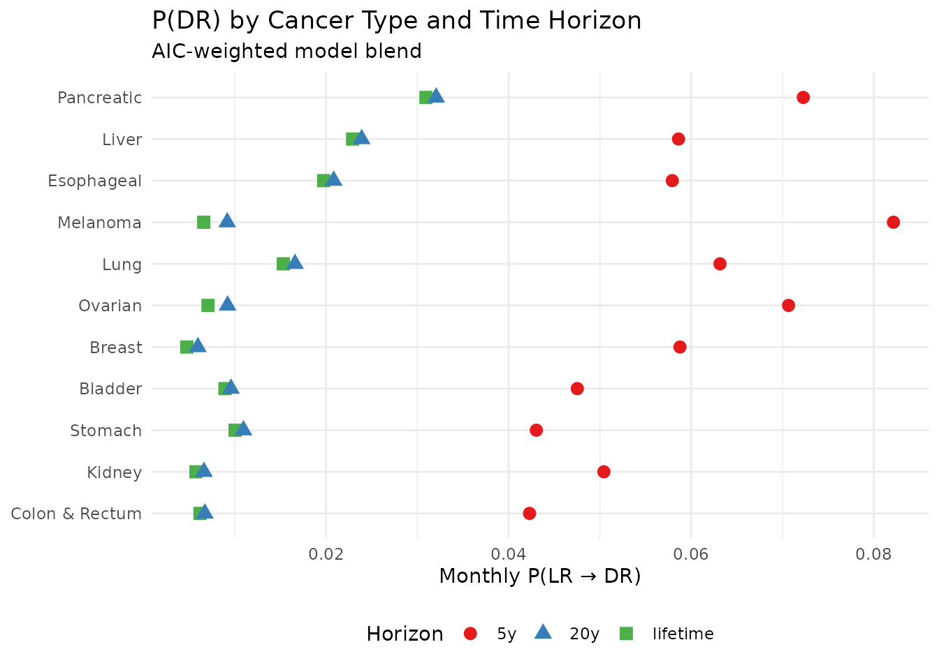

P(DR) across scenarios and criteria

---

AIC vs BIC comparison (lifetime horizon)

all_results |>
  filter(scenario == "lifetime") |>
  select(Tumor, criterion, P_DL_approach2) |>
  pivot_wider(names_from = criterion, values_from = P_DL_approach2) |>
  ggplot(aes(x = AIC, y = BIC, label = Tumor)) +
  geom_point(size = 3, colour = "#E41A1C") +
  geom_text(size = 3, vjust = -0.6, hjust = 0.5) +
  geom_abline(slope = 1, intercept = 0, linetype = "dashed", colour = "grey50") +
  labs(
    title = "AIC- vs BIC-weighted P(DR) — Lifetime Horizon",
    x     = "P(LR → DR) under AIC weighting",
    y     = "P(LR → DR) under BIC weighting"
  ) +
  theme_minimal(base_size = 11)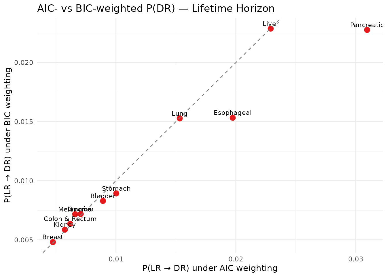

AIC vs BIC — P(DR)

---

Exporting results

# Export combined results to CSV
write.csv(
  all_results,
  file      = "seerSurv_all_results.csv",
  row.names = FALSE
)

# Export base-case to Excel
openxlsx::write.xlsx(
  base,
  file      = "seerSurv_basecase.xlsx",
  sheetName = "Lifetime_AIC"
)

---

Session information

sessionInfo()
#> R version 4.5.3 (2026-03-11)
#> Platform: x86_64-pc-linux-gnu
#> Running under: Ubuntu 24.04.3 LTS
#> 
#> Matrix products: default
#> BLAS:   /usr/lib/x86_64-linux-gnu/openblas-pthread/libblas.so.3 
#> LAPACK: /usr/lib/x86_64-linux-gnu/openblas-pthread/libopenblasp-r0.3.26.so;  LAPACK version 3.12.0
#> 
#> locale:
#>  [1] LC_CTYPE=C.UTF-8       LC_NUMERIC=C           LC_TIME=C.UTF-8       
#>  [4] LC_COLLATE=C.UTF-8     LC_MONETARY=C.UTF-8    LC_MESSAGES=C.UTF-8   
#>  [7] LC_PAPER=C.UTF-8       LC_NAME=C              LC_ADDRESS=C          
#> [10] LC_TELEPHONE=C         LC_MEASUREMENT=C.UTF-8 LC_IDENTIFICATION=C   
#> 
#> time zone: UTC
#> tzcode source: system (glibc)
#> 
#> attached base packages:
#> [1] stats     graphics  grDevices utils     datasets  methods   base     
#> 
#> other attached packages:
#> [1] ggplot2_4.0.2  tidyr_1.3.2    dplyr_1.2.0    seerSurv_0.1.0
#> 
#> loaded via a namespace (and not attached):
#>  [1] sass_0.4.10         generics_0.1.4      lattice_0.22-9     
#>  [4] digest_0.6.39       magrittr_2.0.4      evaluate_1.0.5     
#>  [7] grid_4.5.3          RColorBrewer_1.1-3  mvtnorm_1.3-6      
#> [10] fastmap_1.2.0       jsonlite_2.0.0      Matrix_1.7-4       
#> [13] mstate_0.3.3        deSolve_1.42        survival_3.8-6     
#> [16] purrr_1.2.1         scales_1.4.0        codetools_0.2-20   
#> [19] numDeriv_2016.8-1.1 textshaping_1.0.5   jquerylib_0.1.4    
#> [22] cli_3.6.5           rlang_1.1.7         splines_4.5.3      
#> [25] withr_3.0.2         cachem_1.1.0        yaml_2.3.12        
#> [28] flexsurv_2.3.2      tools_4.5.3         vctrs_0.7.1        
#> [31] R6_2.6.1            lifecycle_1.0.5     muhaz_1.2.6.4      
#> [34] fs_1.6.7            ragg_1.5.1          pkgconfig_2.0.3    
#> [37] desc_1.4.3          pkgdown_2.2.0       pillar_1.11.1      
#> [40] bslib_0.10.0        gtable_0.3.6        glue_1.8.0         
#> [43] data.table_1.18.2.1 Rcpp_1.1.1          statmod_1.5.1      
#> [46] systemfonts_1.3.2   xfun_0.57           tibble_3.3.1       
#> [49] tidyselect_1.2.1    knitr_1.51          farver_2.1.2       
#> [52] htmltools_0.5.9     labeling_0.4.3      rmarkdown_2.30     
#> [55] compiler_4.5.3      S7_0.2.1            quadprog_1.5-8